Hazardous location identification for head-on collisions with roadside assets and objects: A deep learning approach
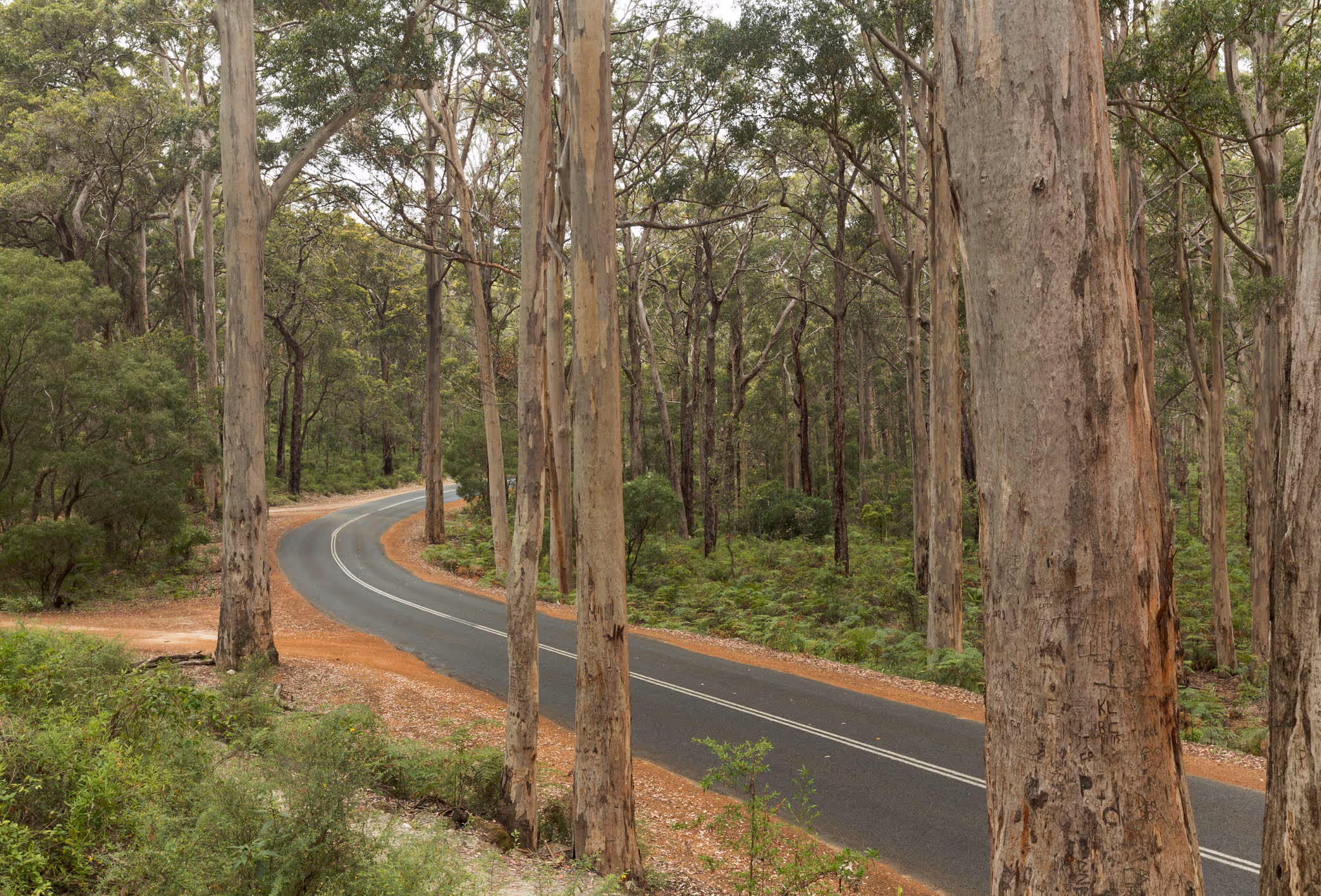
In road safety, the “killer tree” problem refers to a head-on collision with a pole/tree and contributes to 30-50% of Australian road fatalities (Morris et al. 2001). As such, hazardous trees are a component of the International Road Assessment Programme (iRAP) star rating process for road safety inspections, impact assessments and designs.
In road safety, the “killer tree” problem refers to a head-on collision with a pole/tree and contributes to 30-50% of Australian road fatalities (Morris et al. 2001). As such, hazardous trees are a component of the International Road Assessment Programme (iRAP) star rating process for road safety inspections, impact assessments and designs. However, repeat iRAP ratings of a specific road segment are performed less frequently than the rate at which vegetation can grow from a non-hazardous size to a hazardous one (e.g. possible in 3-12 months). Additionally, the iRAP rating process is applied manually, which is time consuming and costly.
Developing a lower-cost, more innovative and faster network monitoring system is considered highly desirable. A promising approach to achieve this, and better monitor gradually changing assets, is to enable automated and semi-automated network monitoring with artificial intelligence (AI) and machine learning (ML). As such, the Australian Road Research Board (ARRB) was commissioned by the Queensland Department of Transport and Main Roads’ (TMR) Spatial Labs to develop an end-to-end model for detecting and classifying road assets and vegetation that detects and maps killer tree hazards.
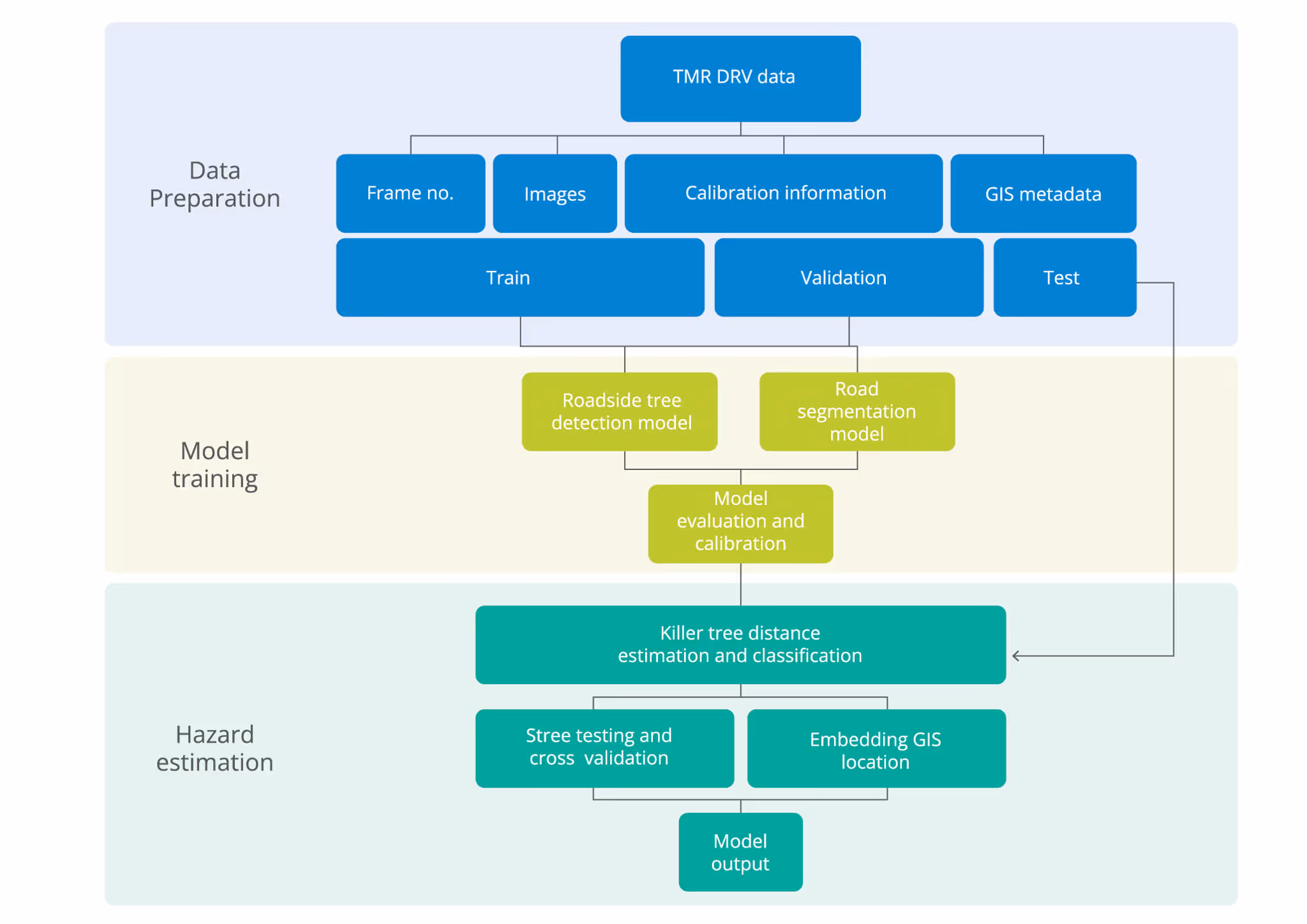
By implementing state-of-the-art deep-learning algorithms for an efficient classification and detection system, and noting that the identification of killer tree hazards is a three-level process (Figure 1), the methodology proposed by ARRB will help identify killer trees and flag the geo-locations in a Geographic Information System (GIS). This will facilitate infrastructure management agencies to act against noted hazards and carry out necessary treatments.
Figure 1: Three-level process to identifying killer tree hazards using AI/ML
The challenges in existing data collection and processing methodologies used for road safety and asset management were also considered (Table 1). To overcome the challenges to detecting hazardous locations with the presence of roadside objects (e.g., killer trees), this project pursued the development and evaluation of an AI tool.
Challenge
Description
Cost
Raw data collection, annotation and post-processing for ratings require intensive, manual human monitoring (e.g., for identifying defects and/or road network changes) of thousands of kilometres of footage and are thus costly.
Time
Surveys are performed less frequently than required to account for significant vegetative growth. Increasing survey frequency for more up-to-date information would be, timewise, almost impossible to process manually.
Data
Advanced automated technologies collect large amounts of raw data, which is costly to ingest and process on the backend.
Automation
Detection and classification of hazards: most road ratings are assessed manually and not all the safety attributes can be captured automatically.
Table 1: Data collection challenges/gaps
Data description
Digital Video Road (DVR) is a type of video data created from the road data annually collected by ARRB for all state-controlled roads in Queensland. The DVR data consists of two sets of data files:
Spatial video - image footage of recorded locations at 10 m intervals, and
Navigational (NVG) - calibration metadata and the GIS information associated with each video frame.
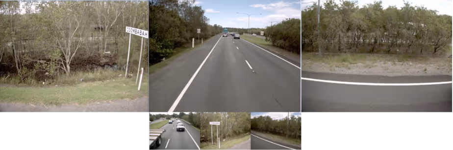
Spatial video data comprises frames taken at 10 m intervals from 7 different directions - forward, left, right, rear, left side, right side, and the road surface (generated at 5 m intervals). Depending on the surveyed road section’s length, multiple files are generated for each camera. Figure 2 shows an example of all captured directions when viewing files in a DVR viewer.
Figure 2: Example of video data when opened in a DVR viewer
NVG files store the metadata and attributes listed in Table 2, including those used for each DVR (e.g., road name, lane number, etc…). NVG file data, including for road chainages, GPS coordinates, altitude and frame numbers, are collected at 10 m intervals and at 5 m intervals for the NVGX file (i.e. NVG file with additional information from extra cameras and the road surface video).
NVG file attributes and metadata
Survey vehicle type
Codec
Calibration plane type
Flip image
Survey date
Compression level
Calibration point type
Chainage
Survey time
Offset forward
Pixel X
Section ID
Road name
Offset right
Pixel Y
Sectional chainage
Carriageway number
Height
Distance X
Latitude
Lane
Pan
Pan
Longitude
Direction
Tilt
Distance Z
Altitude
Description
Resolution
Calibration point
Frame number for each camera
Comment
Field of view
Calibration plane
Camera name (direction)
Calibration
Filenames (AVI files)
Table 2: List of NVG file attributes and metadata
Methodology
The project proposed that by using the front view camera’s DVR image data, training of a custom model could be undertaken for detecting killer trees and reporting the geographical location. An overview of the development process is described in this article, with Figure 3 below depicting the block diagram for the proposed methodology.
Figure 3: Proposed methodology
For data preparation, data is divided into training and testing. The latter includes annotating tree trunks and driveable paths using annotation tools such as OpenVINO's CVAT1 (utilised in this project). For ease of use and precision, tree trunks were detected utilising polygon coordinates/polygon masks, which allowed detection to the pixel and thus more precise distance estimations. Figure 4(a) shows an example of data annotated in this way. Upon annotating a few images, the data is exported with the polygon coordinates.
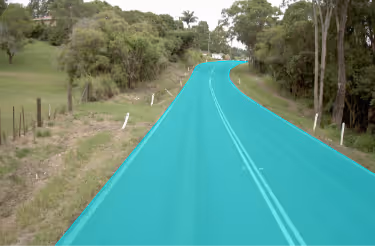
To determine the distance of a given object to the road, the boundaries of the road must be identified. While different approaches can be used for this road segmentation, it was decided to use the same object detection pipeline developed for tree trunk detection. Figure 4(b) shows an example of a labelled road used to train the model.
(a)
(b) Figure 4: Example of annotated (a) tree trunks, and (b) road segmentation using CVAT
Detection model, algorithms and architectures
Transfer learning
Training a model from scratch requires extensive training data and resources. To reduce time and resources in developing a custom model, the project made use of transfer learning. This process is “the improvement of learning in a new task through the transfer of knowledge from a related task that has already been learned.” (Soria et al. 2009).
The most vital task for this project is detecting tree trunks along the road corridor. To do this, an open-source project mask regional-based convolutional neural network (R-CNN)2 was utilised, which employed in its method feature pyramid networks, along with a ResNet101 backbone, to identify features. Then, a pre-trained model on the Microsoft Common Objects in Context (MS COCO) dataset (Lin et al. 2015) was utilised to identify anchors within images. The last layer of the model was then trained on the project data to identify tree trunks from these anchors.
Using this transfer learning process, the tree trunk and road segmentation model was trained by annotating 180 images, a relatively small data set, saving much time.
Tree trunk detection
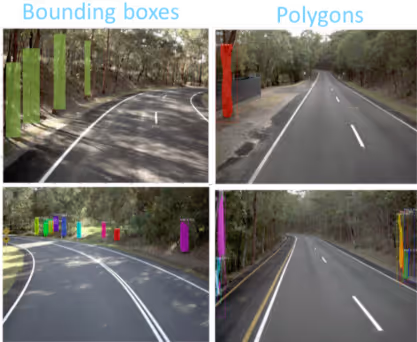
Training data was exported with the polygon coordinates and the final layer of the model was then trained on the small tree trunk dataset. Figure 5 shows tree trunk detection results when bounding boxes or polygons were used for data annotation. The result shows that the trunks' edge detection using polygons outperforms the bounding boxes, so the project progressed with polygon annotation.
Figure 5: The impact of bounding boxes and polygons annotation on the trunk detection
Road segmentation
For road segmentation, an off-the-shelf MobileNet (Howard et al. 2017) model trained on the CityScapes dataset (Cityscapes Dataset 2022) was identified for use in the project. However, the available model wasn’t deemed precise enough due to the inclusion of the road shoulder and gravel paths in its mask (Figure 6).
Figure 6: An example of using the shelf semantic segmentation on the DVR data using MobileNet. Source: (Howard et al. 2017)
To overcome this, a small data set was labelled and used to train the available model based on polygons with outside road lines in the labelling. This allowed the model to identify the drivable path of the road without including the shoulder. This was theorised to have better precision in road width estimation, allowing the width of any given road segment to be assumed as 7 m, based upon an average 2-lane road. Figure 7 shows the successful road segmentation and tree trunk detection using the proposed model.
Figure 7: Successful road segmentation and tree trunk detection using proposed transfer learning
Hazard distance estimation model
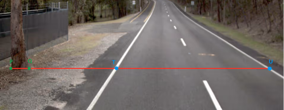
To estimate the distance of an object to the road, a pixel-distance ratio is used. As a typical road lane is 3.5 m, and the roads used as training inputs had two lanes, a driveable width of 7 m was assumed. Figure 8 shows points P and Q indicating the edges of the tree, and points T and U indicating the edges of the road. The difference in X-coordinate pixels was used to determine the distance of the tree, and its width, by calculating the pixel-driveable width ratio at that distance.
Figure 8: Image showing the distance estimation procedure.
To determine whether a tree is dangerous, iRAP ratings (IRAP 2021) are applied. These ratings provide three categories of the hazardous trees, all with trunks greater than 10 cm in diameter. In decreasing order of danger:
Trunks closer than 1 m to the road
Trunks 1 to 5 m from the road
Trunks 5 to 10 m from the road.
Detected trees are categorised based on calculated widths and distances, then multiplied by an extra 15% to account for any errors from the road to determine the danger category. These are then reported by the program along with real-world location coordinates and a survey date. Table 3 provides a program output example for both a location with, and one without, an identified killer tree based on iRAP rating for trunks greater than 10 cm in diameter and closer than 1 m to the road.
Date
Diameter (m)
Distance from road (m)
ID
Latitude
Longitude
Hazard category
11/06/2021
0.2894
0.7165
104
-27.6499
153.2307
i
11/06/2021
0.1568
6.2048
105
-27.6500
153.2306
iii
Table 3: Sample trunk detection GIS report and associated attribute
Evaluation result and discussion
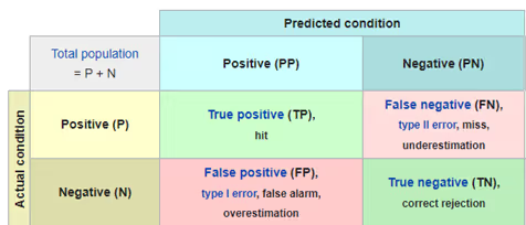
The evaluation of the end-to-end performance of the proposed model (Figure 3) was undertaken by computer vision and pattern recognitions to compare the predicted vs actual condition outcomes of the model. Accuracy of the model, determined by the ratio of the total number of correctly identified samples to the total number of samples, was calculated using a confusion matrix (Table 4).
Table 4: Binary classification confusion matrix
Where: TP = correctly labelled as acceptedTN = correctly labelled as rejected
FP = incorrectly labelled as acceptedFN = incorrectly labelled as rejected
The matrix provides insight into the system's overall performance, including the model sensitivity, specificity, miss rates and fall-out rates (Table 5). These metrics are reported on a range of 0 to 1 (respectively low to high). In general, a high sensitivity and specificity rate show that the system is good in killer tree detection and correctly rejects objects that are not killer trees.
Performance Measure
Description
Calculation
Sensitivity
True positive rate (TPR): how well true positives can be identified.
High outcome = Model is good at detecting killer trees.
TPR = TP / (TP + FN)
Specificity
True negative rate (TNR): how well true negatives can be identified.
High outcome = Model is good at identifying when there are no killer trees.
TNR = TN / (TN + FP)
Miss rate
FP ratio: how often the model is missing object identification.
High outcome = Model is incorrectly classifying non-killer trees as killer trees.
FPR = 1 − TNR
Fall-out rate
FN ratio: how often the model is incorrectly identifying objects.
High outcome = Model is missing out on identifying a lot of killer trees.
FNR = 1 − TPR
Table 5: System performance measures
Evaluation results for selected use cases
To evaluate the proposed algorithm, reported crash data from TMR3 and ARRB's road survey repository were leveraged to identify locations with prevalent trees and a type of crash identified as “off carriageway hit object”. From this, Mt Cotton was selected as a control site and route No. 414_1 was selected as a ”hazardous tree in driving scene” use case.
To avoid biasing outcomes, the evaluation data had not been seen before by the model. A total of 135 scenes were manually annotated using visual observation and binary decision making to find a trunk and decide on the killer tree potential of the object in each image.
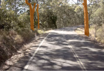
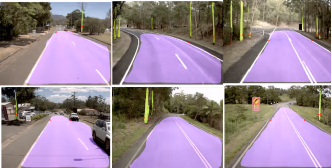
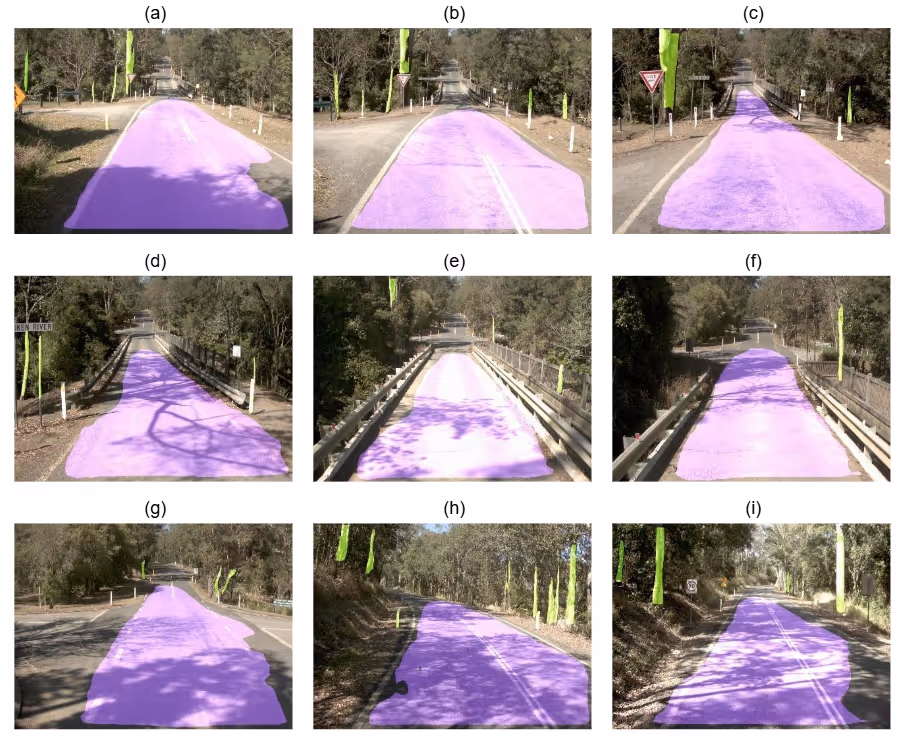
Figure 9 shows the qualitative results of the proposed detection model on sequential images of a test road. The result indicates a consistent detection from one frame to the next. It is also observable that signs, bars or pillars are sometimes detected as a tree trunk. These false detections do not pose significant issue for the proposed end-to-end model due to size, height and dimension. The manual annotation shows that TP= 89 and FP = 7 for the selected samples shows the 96% accuracy of tree trunk detection using Mask-RCNN.
Figure 9: qualitative result on road segmentation (purple) and tree trunk detection (green) while driving. (a) to (i) are sequential video frames
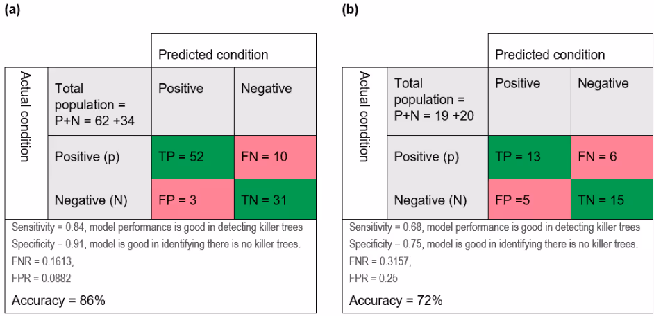
The overall performance of the proposed method on the control and use case sites was evaluated to give an accuracy of 86% and 72% respectively, both acceptable performance levels. Overall, the proposed system was noted to have a high sensitivity and specificity, justifying the proposed model approach in detecting killer trees. The evaluation results for the selected use cases are provided in Table 6.
Table 6: Performance evaluation of the proposed model for (a) Mt Cotton and (b) Route No. 414_1 use cases
Concluding remarks
By utilising deep-learning algorithms, a proof-of-concept, end-to-end model for the detection and classification of killer trees was developed with promising evaluation results. To scale up the proposed model to cover entire road networks, and maintain quality datasets on killer trees, further evaluation is required. The system would also need training through more meaningful/larger datasets.
Future research relies on more efficient data annotation. Although only 180 samples were used and achieved acceptable results (96% in detecting tree trunks), data annotation is still an extensive task. Aggregation of reported incident data with DVR is a complex task and proper data ingestion is required to integrate the proposed model into current safety datasets. As such, generating a data ingestion framework to undertake data annotation in a semi-automated way would be more appropriate for large-scale deployment. Additionally, the proposed data engine could be used to detect other assets such as signs, barriers, lane markings and traffic signs, to generate an inventory system.
Acknowledgment
This work was funded by Queensland Transport and Main Roads (TMR) as part of TMR Spatial Labs program 2022. The authors would like to thank FrontierSI for their inputs on this project.
References
Morris, A, Truedsson, N, Stallgardh, M & Magnisson, M, 2001, Injury Outcomes in Pole/Tree Crashes.pdf, viewed 23 September 2022, <https://acrs.org.au/files/arsrpe/RS010004.pdf>.
Cityscapes Dataset 2022, Cityscapes Dataset – Semantic Understanding of Urban Street Scenes, viewed 23 September 2022, <https://www.cityscapes-dataset.com/>.
Howard, AG, Zhu, M, Chen, B, Kalenichenko, D, Wang, W, Weyand, T, Andreetto, M & Adam, H 2017, 'MobileNets: Efficient Convolutional Neural Networks for Mobile Vision Applications', arXiv:1704.04861 [cs], arXiv, , , no. arXiv:1704.04861, viewed 23 September 2022, <http://arxiv.org/abs/1704.04861>.
IRAP 2021, Star Ratings, iRAP, viewed 26 September 2022, <https://irap.org/rap-tools/infrastructure-ratings/star-ratings/>.
Lin, T-Y, Maire, M, Belongie, S, Bourdev, L, Girshick, R, Hays, J, Perona, P, Ramanan, D, Zitnick, CL & Dollár, P 2015, 'Microsoft COCO: Common Objects in Context', arXiv:1405.0312 [cs], arXiv, , , no. arXiv:1405.0312, viewed 23 September 2022, <http://arxiv.org/abs/1405.0312>.
Soria, O, Emilio, Mart¡n, G, Jos‚ David, Marcelino, M-S, Rafael, M-B, Jose & Jos, SL, Antonio 2009, Handbook of Research on Machine Learning Applications and Trends: Algorithms, Methods, and Techniques: Algorithms, Methods, and Techniques, IGI Global.
Dr Sepehr Dehkordi
Senior Engineer
NTRO
Dr Charles Karl
National Technical Leader - Transport Systems
Trevor Wang
Senior Professional
NTRO
Macgregor Buckley
Data Scientist
Toronto-Dominion Bank
Interiew
Hazardous location identification for head-on collisions with roadside assets and objects: A deep learning approach